
Risk Matrix Modification Procedures
- An important preliminary note: existing "w-if-..." worksheet line items will not be updated by these risk matrix revisions. Only subsequently assigned questions will result in "w-if-..." line items containing the revised risk matrix and calculation. This behavior is due to conditional color formatting and risk matrix data that is copied initially from the hidden template worksheet when a question is assigned to a "w-if..." worksheet.
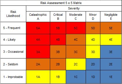
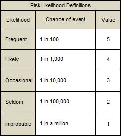
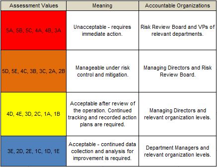
- Let's start with the Matrix worksheet to plan our revisions. Here is the default Risk Matrix chart, Likelihoods chart, and Assessment Values chart.
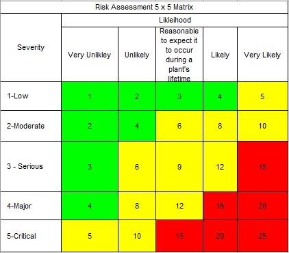
- These are the revisions we performed for planning our new risk matrix. Note, only the Risk Matrix and Assessment Values charts were changed. The Likelihoods chart remains the same.
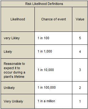
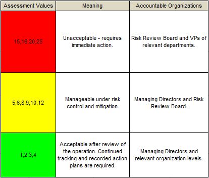
- Next, we move on to changing the actual Risk Matrix data for the x and y-axis. These values are used to populate the dropdown lists, Likelihood and Severity, used in the risk calculation of each line item/question within a "w-if-..." worksheet. They are also used in the Template hidden worksheet. Please see the Lookup Tables worksheet for the following two tables. You may need to horizontally scroll to find the tables within the worksheet. Below are images of the default tables.
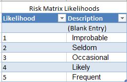
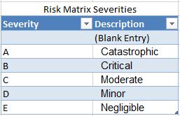
- These are the revisions we performed. Notice we performed significant edits to both tables.
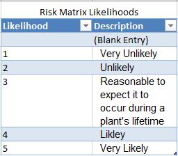
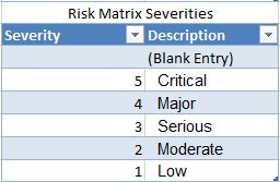
- Next, we need to modify the conditional formatting used for dynamically setting each Risk cells' color. This conditional formatting is stored in the Template worksheet that is typically hidden. You may right-click on any worksheet tab, choose Unhide and then, choose Template to unhide the worksheet.
- After unhiding the Template worksheet, please select the Risk cell and choose Conditional Formatting -> Manage Rules from the Styles section within the ribbon. Here is an image of the default rules along with the Edit dialog displayed for the first rule.
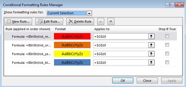
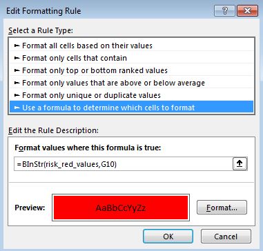
Note, the above formula refers to a named range, risk_red_values, we will not use these default named ranges within our modified version. - Next, we modify each conditional formatting rule to achieve our new color scheme based on the cell's value. Here is an image of the revised rules along with the Edit dialogs displayed for all three rules.
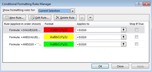
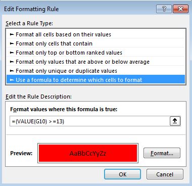
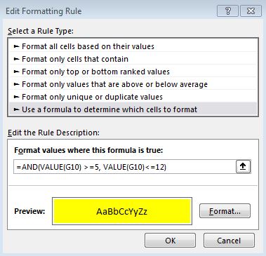
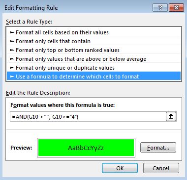
- Plese Hide the Template worksheet when finished with the modifications.
- Finally, within our workbook VBA project, we need to edit the formula for assessing the Risk value based on the Likelihood and Severity. We go to the Developer tab, click the Visual Basic button within the ribbon, and then we should see the workbook VBA project that should look something like this when expanded.
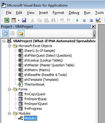
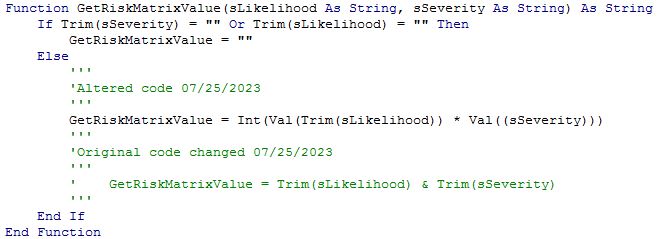
- Next, double-click on Module1 under modules and locate the following function GetRiskMatrixValue(). This is an image of the original function that concatenates the Likelihood (alpha value) and Severity (numeric value).

- Here is our revised function that multiplies the Likelihood and Severity (x and y-axis) numeric values and returns the product as the Risk value. Note, I simply "commented out" the original code. See below.
Visit the product page for our What-If Automated Excel Spreadsheet